Every capacitance or FDR soil moisture sensor ships with a factory curve, and every factory curve was built on a soil that is not yours. The Arizona Extension guide to maintaining and calibrating field-installed soil and plant moisture sensors is blunt about why: soil texture, salinity and temperature all shift what the same probe reports for the same amount of water, and sensors drift with age regardless. Sensor-specific and site-specific calibration are what actually fix the reading, not a firmware update. Doing that calibration properly means catching one physical event on your own ground: the point where a saturated soil finishes draining and settles into what agronomists call field capacity.
This piece walks through that event step by step, with the number that governs each step, because soil moisture sensor calibration is not a settings menu, it is a small field experiment you run once per soil type you manage.
Measured by NuaSense weather stations and soil probes on Kenyan farms, over the period stated with each figure. Past readings, not a forecast.
The event you are trying to catch
Field capacity is defined by the Oregon State Extension guide to soil moisture monitoring as the relatively stable water content a soil settles at after saturation, once gravitational drainage has slowed to something close to negligible. It sits at a soil moisture tension of roughly -10 to -33 kPa depending on texture, sandy soils toward the wetter end of that suction range, clay soils toward the drier. That range is wide on purpose. Nobody can hand you a single field capacity number without knowing your soil, and neither can we.
What matters for calibration is that field capacity gives you a real, physically anchored upper reference point. Below it the soil is drying out under root uptake and evaporation, a process you can watch for weeks. The transition into that drying phase, the moment gravity stops doing the work and the crop takes over, is the one moment worth catching with both a sensor reading and an independent measurement in hand.
Step one: flood a patch and let gravity finish its work
Pick a spot with your probe already installed, undisturbed, ideally the same spot you plan to trust all season. Apply enough water to saturate the profile past where the probe reads, not a light irrigation pass. The soil needs to be genuinely waterlogged at depth for the drainage phase that follows to be meaningful. On a heavy clay block this takes longer to achieve and longer to drain than on a sandy loam, which is the entire reason texture sits at the centre of every calibration source in this piece.
Once ponding disappears from the surface, drainage inside the profile continues invisibly for one to three days depending on texture and depth, a range the extension literature gives qualitatively rather than as a fixed count of hours. This is the part growers skip: they flood, wait a morning, and take a reading while the soil is still actively draining rather than settled. A reading taken mid-drainage is not field capacity, it is just a wet soil in transit, and calibrating against it fixes your curve at a point that will never repeat.
Step two: read the sensor and pull a physical sample at the same hour
Once drainage has visibly slowed, day two or three after saturation is a reasonable window to check, log the sensor's raw output at that exact moment. Then take a physical soil core from beside the probe, at the same depth the sensor reads, and seal it immediately. The Arizona guide describes this as the core of field calibration: collect a sample, weigh it, dry it, and calculate volumetric water content independently of anything the sensor reported. The sensor reading and the physical sample have to come from the same hour and the same depth or the comparison is worthless.
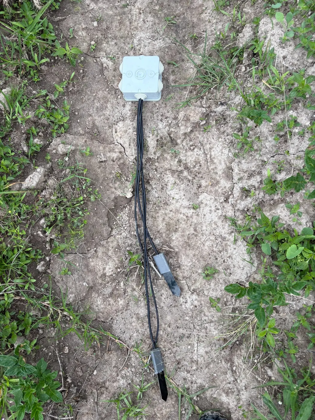
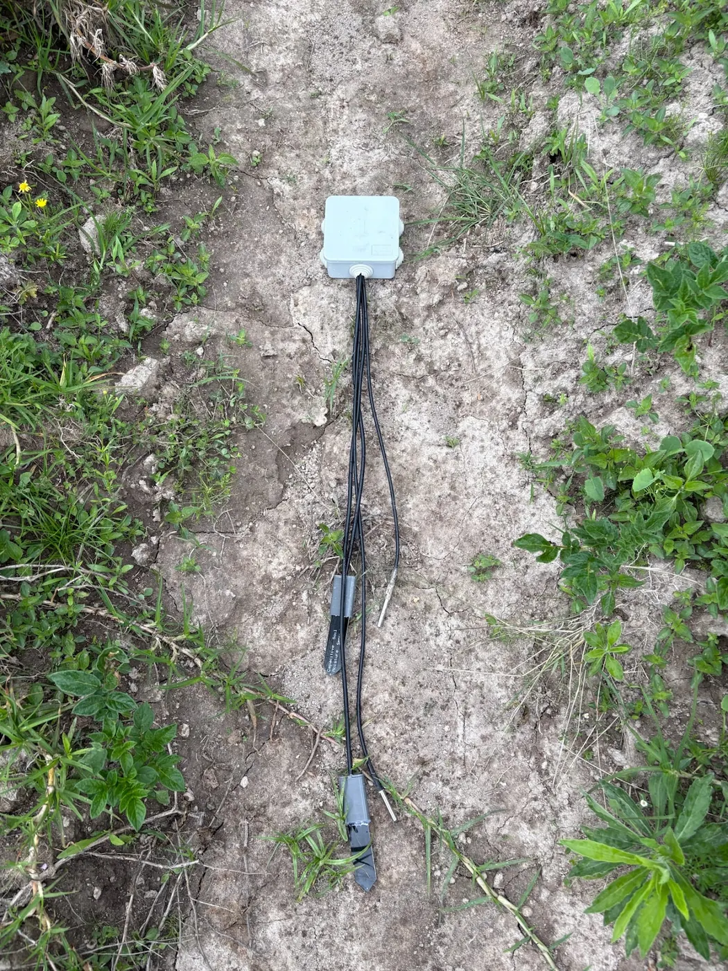
On our own deployed probes, which read at a shallow and a deeper depth chosen per installation by crop and rooting pattern, this means pulling two cores, one matched to each depth, if you want to calibrate both channels rather than assume one curve fits them equally. There is no shortcut here: a single core calibrates a single depth.
Step three: the oven, and why 105 degrees for 48 hours is not negotiable
The gravimetric method described in the study on data-driven calibration of soil moisture sensors under temperature variation is oven-drying the soil sample at 105 degrees Celsius for 48 hours to constant weight. That temperature and duration are specific for a reason: lower temperatures leave bound water in the sample and inflate your measured moisture, shorter durations risk stopping before the sample has actually reached constant weight, especially on a clay-heavy core that holds water more tightly than sand. If you do not have access to a lab oven capable of holding 105 degrees for two full days, this step is the one place in the whole process where a shortcut genuinely corrupts the result, not just introduces noise.
Weigh the sample wet, dry it, weigh it again. The difference in mass divided by the dry mass gives gravimetric water content as a fraction. That fraction is not yet the number you compare against the sensor. It needs one more conversion, and it is the conversion most growers skip.
Step four: turning grams into a percentage that means anything
Gravimetric water content is a mass ratio. Sensors and irrigation decisions run on volumetric water content, a volume ratio, and the two are only the same number if the soil's bulk density happens to equal 1.0 g per cubic centimetre, which it almost never does. The Oregon State guide gives the conversion directly: volumetric water content equals gravimetric water content multiplied by bulk density. Typical bulk density figures from the Arizona guide run 1.4 to 1.7 g/cm³ for sandy soils, 1.2 to 1.5 g/cm³ for loamy soils, and 1.0 to 1.3 g/cm³ for clay soils.
Take a loamy soil at the middle of that range, bulk density 1.35, with a gravimetric water content of 0.20 from your oven test. Volumetric water content works out to 0.20 times 1.35, which is 0.27 cm³/cm³. That is the number that goes against your sensor's raw reading at the field capacity moment, not the 0.20 you read off the scale. Oregon State also gives a useful sense check for that figure: a volumetric water content of 0.25 cm³/cm³ across a 12-inch root zone stores 3 inches of water, so a small error in bulk density translates directly into an error in how much water you think a full root zone actually holds.
Step five: build the curve, or at least the one point you have
One paired reading, sensor output against volumetric water content, gives you one point on a calibration curve. That single point tells you the sensor's error at field capacity, which is genuinely useful, but it is not a curve. A proper curve needs points spread across the moisture range, from field capacity down toward the dry end. A Kenyan-fabricated low-cost capacitive soil humidity sensor project, run at the University of Eldoret and documented in its fabrication and calibration study, calibrated capacitance against gravimetric water content as a third-degree polynomial across four soil texture classes, with correlation coefficients between 0.95 and 0.99. That is what a full curve looks like: multiple points, a fitted shape, and a fit quality you can actually check.
Nobody expects a commercial farm manager to run a four-texture polynomial study. What is worth taking from that Eldoret work is the shape of the exercise: capacitance sensors do not respond linearly to water content, and a single field capacity anchor plus an assumed straight line to zero will misrepresent the middle of your moisture range, exactly where most irrigation decisions actually happen. If field capacity is the only anchor you can afford to catch this season, treat it as one point, log it, and add a second one at a visibly drier moment before you trust the curve for scheduling.
Where temperature quietly wrecks the whole exercise
The same PMC study tested FDR sensor response across 0 to 45 degrees Celsius, using soil from the 0 to 20 cm tillage layer at three fixed moisture levels: 9.58, 18.25 and 27.01 percent, set by soil mixing. Readings varied significantly across that temperature range at every one of those moisture levels. That range was chosen to cover the environmental swing during wheat and corn growth in Northern China, not Kenya, and it is worth naming that gap directly rather than pretending the figures transfer whole.
What does transfer is the mechanism. A capacitance sensor reads the dielectric behaviour of the soil-water mixture, and that behaviour shifts with temperature independently of how much water is actually there. Our own network's soil temperature data show this is not a small effect to ignore: across 3 probes over the same August period, soil temperature averaged 16.5 degrees Celsius, but the two depths behaved differently, one moving through 1.9 degrees over the month and the other through 2.9 degrees, roughly one and a half times the swing. If your calibration reading and your field capacity reading were taken a month apart at noticeably different soil temperatures, part of the difference you are attributing to moisture change is actually a temperature artefact, and there is no way to separate the two after the fact without a temperature-aware model like the MARS and GPR approaches the same PMC study used.
Why a curve fitted on one block does not travel to the next
The PMC study's central finding, after testing fixed-form polynomial equations against data-driven models like multivariate adaptive regression splines and Gaussian process regression, was that the data-driven models outperformed fixed polynomial equations at capturing the actual relationship between measured and true soil moisture, precisely because that relationship is not a clean fixed shape once temperature and soil variation are both in play. The practical read for a Kenyan farm running several blocks: a curve built on your black cotton plot has no business being applied to your neighbouring sandy loam parcel, even with the same probe model and the same firmware. A soil moisture reading means nothing until you know three other numbers, and texture is one of the three that has to be established per block, not assumed from one calibration run.
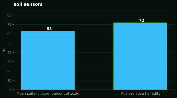
This is also why our own soil moisture sensors report relative moisture as a percentage of sensor scale rather than a calibrated volumetric figure straight out of the box. Across our network, readings average 63 percent of scale with most readings between 18 and 92 percent over a recent month. That is a usable number for tracking whether a block is trending wetter or drier, but it is deliberately not presented as m3/m3, because doing that honestly requires exactly the site-specific gravimetric work described above, done on your soil, not assumed from a factory curve.
The low-cost alternative that skips the oven entirely
Not every farm has lab access, and the AICCRA report on tech-backed irrigation in Eastern and Central Africa documents a simpler route that has already reached real farms. The Chameleon sensor, part of the VIA toolkit first introduced in Africa in 2016 through a CSIRO and ACIAR partnership, skips a numeric calibration entirely and reports a colour: blue for too wet, green for adequate, red for too dry. By 2024 more than 87,000 of these sensors had reached partners across more than 24 countries, and farmers using the wider VIA toolkit, which also includes a wetting front detector, nitrate strips and an EC meter, reported real income gains: Ahmed Saturday moved from USD 285 to USD 6,564 on one acre of cabbages, rice and maize, and one farmer cut irrigation time in half while saving roughly USD 5.5 a week.
Those figures come from Uganda and describe specific farmers, not a typical outcome, and they should not be read as a promise transferable to a Kenyan block. What is transferable is the design choice: a colour-coded threshold sensor sidesteps the entire gravimetric exercise this piece has walked through, at the cost of precision. If your decision is genuinely binary, irrigate or don't, a Chameleon-style threshold is defensible. If you are trying to hit a run time calculated from a measured infiltration rate, the kind of arithmetic covered in why your irrigation run time is wrong without a measured soil infiltration rate, a colour band will not give you the resolution that decision needs.
Standardisation: the calibration most farms should actually run
The Arizona guide names a practical middle path between full lab calibration and no calibration at all: sensor standardisation, which means monitoring the sensor's own readings before and after an irrigation event rather than converting every reading to an absolute volumetric figure. You are not asking what the soil's water content is in cm³/cm³. You are asking whether this irrigation moved the reading by the amount you expect, and whether the post-irrigation plateau lands in roughly the same place each time.
This is closer to how most commercial farms actually use continuous soil sensors day to day, and it is the approach our products are built around: relative moisture on a fixed scale, tracked over time per probe, rather than a one-off absolute figure that needs a lab to validate. The NuaSense overview of smart irrigation in Kenya covers how drip systems and soil probes work together under this relative-tracking model, which is the practical answer for most operations that cannot run an oven-and-scale calibration on every block they manage but can absolutely watch whether a reading rises after irrigation and falls at a rate consistent with the crop's stage.
Failure mode: taking the reading during drainage, not after it
The single most common way this exercise goes wrong is impatience. A grower floods a plot, checks back the same evening, sees a high stable-looking number, and logs it as field capacity. It is not. Drainage inside a saturated profile continues well past the point where the surface looks dry, and a reading taken too early sits somewhere between saturation and field capacity, a moving target rather than the settled reference point the whole calibration depends on. There is no fixed hour that works across all textures; the only fix is watching the sensor's own trace flatten before you trust it.
Failure mode: a sample that does not match the sensor's depth or hour
A gravimetric sample taken from a different depth than the probe reads, or hours away from when the sensor logged its reading, cannot be reconciled with that reading no matter how carefully the oven step is done. Soil moisture changes fast enough near the surface, and depth profiles differ enough between the shallow and deeper zones a probe covers, that a same-day mismatch of even a few hours can shift the true value more than the sensor's actual error does. Match depth and hour exactly, or do not bother comparing the two numbers at all.
Failure mode: physical damage nobody notices until the data looks wrong
The Arizona guide flags trampled probes and damaged cables as a routine cause of bad data, and it is an unglamorous failure that calibration work will not fix, because the sensor was never reading cleanly to begin with. A cracked cable insulation, a probe knocked out of full soil contact by cultivation equipment, or a rodent-chewed lead all produce readings that look like drift or texture variation but are actually mechanical failure. Before spending a weekend on an oven and a scale, walk the probe line and check that every unit is still seated the way it was installed. Drift correction on a physically damaged sensor is calibration wasted on a fault that a field visit would have caught in five minutes.
Failure mode: trusting one calibration point for a whole season
Sensors drift, and the Arizona guide is explicit that this requires frequent recalibration rather than a single reference reading trusted indefinitely. A field capacity event caught in April tells you the sensor's behaviour in April's soil temperature and April's soil structure, not August's. The drought.gov guidance on soil moisture data quality makes the same point from the data-quality side: calibration practice differs by the tier of data quality you actually need, and a farm running scheduling decisions off the sensor needs a higher tier, and more frequent rechecking, than one just watching for gross wet or dry swings. Treat the field capacity event as something to catch again each season, not a number you bank once and forget.